How To Use VLOOKUP In Google Sheets – Step By Step Explanation

Introducing the club for anybody who ever ran through a gigantic pile of data in Google Sheets, searching desperately to find some magical figure. Do not despair: there is a nifty little thing called VLOOKUP that can transform you from spreadsheet soccer mom to data-wizard in 10 minutes. Grab your coffee & put on your thinking cap and let’s deep delve into the VLOOKUP World with a checking pinch of Humor.

What is VLOOKUP?

Lets take a step back — VLOOKUP means Vertical Lookup. A simple way to think of this is like the search function in a spreadsheet, but restricted only to one column. Imagine it as your built-in detective who is very good at finding things in a vertical list but absolutely nothing about what do you if the list turns sideways.

Simply put, VLOOKUP helps to locate and will return the value from any other column of this row. Well, picture you have a massive list of all student names and their grades at the end of that year; you want to figure out what grade is for your one single person. Enter VLOOKUP to the rescue!!!

How Does VLOOKUP Work?

The basic Syntax of VLOOKUP is as follows:

plaintext

Copy code

VLOOKUP(search_key, range, index) → the values “False” can be entered accordingly if it is not sorted.

search_key: Value, which we will look for So, the name of some student.

range: The cells range in which there is data. This is where the search key will be searched by VLOOKUP.

index: The ordinal value of the column to return from its range // from here you want output The first column in your range is 1 and the second column is 2 etc.

[is_sorted]: An optional argument used to specify if the first column of the range has been sorted. If you set this to FALSE, VLOOKUP will find an exact match only.

Got it? Great! So, now that we have a little background on some of the terms you are likely to encounter let me give you 5 examples.

Example 1: Student Grades

For example, if you have a sheet with student names in column A and their grades for one test only in Column B your data may look like this:

BabyAlice-100-Bob90-Carol122-David121

It must also mean that you want to know how Bob has fared. Here’s how you’d use VLOOKUP:

Choose the cell where you want the result to appear.

Type formula: =VLOOKUP(“Bob”, A1:B4, 2, FALSE)

Let’s break this down:

“Bob” is the search_key.

You can type in the area where VLOOKUP worked as a chef

2 is the column index we need value to retrieve (column B)

You set an exact match when you type FALSE.

Voila! This is the grade of Bob, so VLOOKUP will return 85. Magic for the real number theorists

For example 2:LOOKUP in Numbers

VLOOKUP will still save your numbers, not names. Imagine you have a table with product IDs and prices:

CD1001$201002$351003$50

Now suppose let’s say you want to find the price for product id 1002 Here’s the VLOOKUP formula:

=VLOOKUP( 1002, C1:D3, 2)

In this example:

1002 is the search_key.

is the range.

Prices are in the 2nd columns

FALSE for an exact match.

This will return $35. That way you will know the cost of this product and not have to search through your whole catalog.

Top Traps and How to Dodge Them

The top of the line can fall and VLOOKUP is no different. Common Problems: What can go wrong and how to fix it

“#N/A” Error

This generally means VLOOKUP was not able to find the search_key Double-check:

Your search_key is spelled properly.

The range is across the correct columns.

Column Index Errors

If the index number is too high or too low, you will receive an error. Ensure the index number is same as your fetching column. The first column in your range is 1, ignore the decimals below.

Sorted Data

You can add TRUE for the [is_sorted] argument if it is, but beware — an otherwise WILL work backwards from there and return you the nearest match to your lookup criterion in case no exact one exists. If an exect match is required, use FALSE instead.

Pro Tips: Advanced VLOOKUP Tricks

Want to become a VLOOKUP wizard instead? I have collated a few tricks which could level up your excel game and make you the Spreadsheet superhero in front of everyone.

Using VLOOKUP with Wildcards

So if you are not aware of the exact value very well, then wildcards can be used for sure.

Asterisk — any character sequence

?? — it replaces any single character.

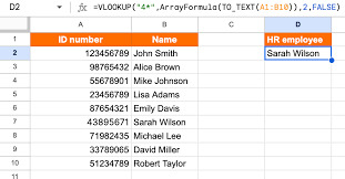
Example, if you want to lookup any student whos name start with “A”, then use as below: =VLOOKUP(“A*”, A1:B4, 2FALSE)

Enhanced VLOOKUPs with Other Functions

You can even make your formulas more powerful by combining VLOOKUP with functions such as IF. Here a sample eg: =IF(VLOOKUP(“Alice”, A1:B4, 2, FALSE) >85, “Excellent”, “Needs Improvement”)

Handling Large Data Sets

For larger data sets please use FILTER or QUERY functions to substitute them. They can take care of advanced circumstances and different criteria increasingly proficiently contrasted with VLOOKUP.

The Next-Level VLOOKUP Troubleshooting

Here is how to suffer less if VLOOKUP does not want you or work as expected.

Check Your Range

Ensure your range extends to all the columns you use in your VLOOKUP function. If the range does not encompass all of relevamt columns, VLOOKUP will locate the best available match but it may be sort of wrong because we couldnt retrieve some related information.

Verify Exact Matches

If you are observing unexpected results, make sure that the [is_sorted] argument is FALSE for exact matches. For unsorted data, this is important.

Double-Check Index Numbers

Make sure the column index is correct. It would be like asking a magician for the rabbit, only to get his hat instead when you found column after nth number was incorrect.

Real-World Uses for VLOOKUP

Now, to wrap it all together and see how exactly VLOOKUP can be a lifesaver in some real-life scenarios.

Party Planning

Consider that you are planning a large-scale event where dietary preferences have been provided with the invitees invited. This way you easily find out who among your guests is a vegetarian, or allergic to peanuts (trust me something like this will save you from disastrous culinary mishaps).

Vacation Planning

When planning a trip and you have a list of destinations, costs and availability — VLOOKUP will help you find exactly which location works with your budget on those dates.

Personal Budgeting

It is a pain in the butt to track your spending, but with VLOOKUP you can easily find all that money went down hole into dining out vs groceries. The answer will finally be revealed “Where did it all go?”

Conclusion:

That is all you have to do in order to use VLOOKUP function on Google Sheets Whether you are fetching student grades, product prices or just want to brag about your new found spreadsheet skills from Thursday work class, VLOOKUP can save your day.

And on that note: VLOOKUP is an amazing function, but surely not the only one in Google Sheets. Keep experimenting and teaching yourself — you know what they say, the more you learn, the stronger your spreadsheets will be. Just remember that if you start to get lost, VLOOKUP is there for the ride as your Batman (or sidekick) ready with a rope whenever you need to fill in those data gaps.

Enjoy spreadsheeting, and may all your data always line up!